Combining 'Traditional' and Text-Based Models to Board Game Ratings
By Brendan Graham in tidy tuesday tidymodels data science
January 26, 2022
Last week I tried out a text based model for the first time. This week I want to continue working with a text based model, but supplement the text data with other non-text predictors. The goal will be to use the board game category (text data) and other non-text data to predict the average board game rating.
Explore the Data
there are 2 tables, one that has the ratings variable we’ll use as the outcome, and the other has some columns to be used as predictors.
ratings
## # A tibble: 21,831 × 10
##      num     id name     year  rank average bayes_average users_rated url
##    <dbl>  <dbl> <chr>   <dbl> <dbl>   <dbl>         <dbl>       <dbl> <chr>
##  1   105  30549 Pandem…  2008   106    7.59          7.49      108975 /boardgam…
##  2   189    822 Carcas…  2000   190    7.42          7.31      108738 /boardgam…
##  3   428     13 Catan    1995   429    7.14          6.97      108024 /boardgam…
##  4    72  68448 7 Wond…  2010    73    7.74          7.63       89982 /boardgam…
##  5   103  36218 Domini…  2008   104    7.61          7.50       81561 /boardgam…
##  6   191   9209 Ticket…  2004   192    7.41          7.30       76171 /boardgam…
##  7   100 178900 Codena…  2015   101    7.6           7.51       74419 /boardgam…
##  8     3 167791 Terraf…  2016     4    8.42          8.27       74216 /boardgam…
##  9    15 173346 7 Wond…  2015    16    8.11          7.98       69472 /boardgam…
## 10    35  31260 Agrico…  2007    36    7.93          7.81       66093 /boardgam…
## # … with 21,821 more rows, and 1 more variable: thumbnail <chr>
details
## # A tibble: 21,631 × 23
## num id primary description yearpublished minplayers maxplayers
## <dbl> <dbl> <chr> <chr> <dbl> <dbl> <dbl>
## 1 0 30549 Pandemic In Pandemic, seve… 2008 2 4
## 2 1 822 Carcasso… Carcassonne is a … 2000 2 5
## 3 2 13 Catan In CATAN (formerl… 1995 3 4
## 4 3 68448 7 Wonders You are the leade… 2010 2 7
## 5 4 36218 Dominion "You are a m… 2008 2 4
## 6 5 9209 Ticket t… With elegantly si… 2004 2 5
## 7 6 178900 Codenames Codenames is an e… 2015 2 8
## 8 7 167791 Terrafor… In the 2400s, man… 2016 1 5
## 9 8 173346 7 Wonder… In many ways 7 Wo… 2015 2 2
## 10 9 31260 Agricola Description from … 2007 1 5
## # … with 21,621 more rows, and 16 more variables: playingtime <dbl>,
## # minplaytime <dbl>, maxplaytime <dbl>, minage <dbl>,
## # boardgamecategory <chr>, boardgamemechanic <chr>, boardgamefamily <chr>,
## # boardgameexpansion <chr>, boardgameimplementation <chr>,
## # boardgamedesigner <chr>, boardgameartist <chr>, boardgamepublisher <chr>,
## # owned <dbl>, trading <dbl>, wanting <dbl>, wishing <dbl>
Using the skimr package we can get a quick understanding of the characteristics of each table.
skimr::skim_to_list(ratings)
Variable type: character
| skim_variable | n_missing | complete_rate | min | max | empty | n_unique | whitespace |
|---|---|---|---|---|---|---|---|
| name | 0 | 1 | 1 | 107 | 0 | 21432 | 0 |
| url | 0 | 1 | 16 | 68 | 0 | 21831 | 0 |
| thumbnail | 6 | 1 | 135 | 139 | 0 | 21816 | 0 |
Variable type: numeric
| skim_variable | n_missing | complete_rate | mean | sd | p0 | p25 | p50 | p75 | p100 | hist |
|---|---|---|---|---|---|---|---|---|---|---|
| num | 0 | 1 | 10915.00 | 6302.21 | 0.00 | 5457.50 | 10915.00 | 16372.50 | 21830.00 | ▇▇▇▇▇ |
| id | 0 | 1 | 118144.78 | 105369.55 | 1.00 | 12308.50 | 104994.00 | 207219.00 | 350992.00 | ▇▂▃▃▂ |
| year | 0 | 1 | 1987.44 | 193.51 | 0.00 | 2001.00 | 2011.00 | 2017.00 | 3500.00 | ▁▁▇▁▁ |
| rank | 0 | 1 | 10916.00 | 6302.21 | 1.00 | 5458.50 | 10916.00 | 16373.50 | 21831.00 | ▇▇▇▇▇ |
| average | 0 | 1 | 6.42 | 0.93 | 1.04 | 5.83 | 6.45 | 7.04 | 9.57 | ▁▁▅▇▁ |
| bayes_average | 0 | 1 | 5.68 | 0.36 | 0.00 | 5.51 | 5.54 | 5.67 | 8.51 | ▁▁▁▇▁ |
| users_rated | 0 | 1 | 866.96 | 3679.82 | 30.00 | 56.00 | 122.00 | 392.00 | 108975.00 | ▇▁▁▁▁ |
skimr::skim_to_list(details)
Variable type: character
| skim_variable | n_missing | complete_rate | min | max | empty | n_unique | whitespace |
|---|---|---|---|---|---|---|---|
| primary | 0 | 1.00 | 1 | 107 | 0 | 21236 | 0 |
| description | 1 | 1.00 | 49 | 16144 | 0 | 21615 | 0 |
| boardgamecategory | 283 | 0.99 | 8 | 216 | 0 | 6730 | 0 |
| boardgamemechanic | 1590 | 0.93 | 8 | 478 | 0 | 8291 | 0 |
| boardgamefamily | 3761 | 0.83 | 13 | 2768 | 0 | 11285 | 0 |
| boardgameexpansion | 16125 | 0.25 | 7 | 18150 | 0 | 5264 | 0 |
| boardgameimplementation | 16769 | 0.22 | 6 | 890 | 0 | 4247 | 0 |
| boardgamedesigner | 596 | 0.97 | 7 | 332 | 0 | 9136 | 0 |
| boardgameartist | 5907 | 0.73 | 6 | 8408 | 0 | 9080 | 0 |
| boardgamepublisher | 1 | 1.00 | 6 | 3744 | 0 | 11265 | 0 |
Variable type: numeric
| skim_variable | n_missing | complete_rate | mean | sd | p0 | p25 | p50 | p75 | p100 | hist |
|---|---|---|---|---|---|---|---|---|---|---|
| num | 0 | 1 | 10815.00 | 6244.48 | 0 | 5407.5 | 10815 | 16222.5 | 21630 | ▇▇▇▇▇ |
| id | 0 | 1 | 118133.09 | 105310.42 | 1 | 12280.5 | 105187 | 207013.0 | 350992 | ▇▂▃▃▂ |
| yearpublished | 0 | 1 | 1986.09 | 210.04 | -3500 | 2001.0 | 2011 | 2017.0 | 2023 | ▁▁▁▁▇ |
| minplayers | 0 | 1 | 2.01 | 0.69 | 0 | 2.0 | 2 | 2.0 | 10 | ▇▁▁▁▁ |
| maxplayers | 0 | 1 | 5.71 | 15.10 | 0 | 4.0 | 4 | 6.0 | 999 | ▇▁▁▁▁ |
| playingtime | 0 | 1 | 90.51 | 534.83 | 0 | 25.0 | 45 | 90.0 | 60000 | ▇▁▁▁▁ |
| minplaytime | 0 | 1 | 63.65 | 447.21 | 0 | 20.0 | 30 | 60.0 | 60000 | ▇▁▁▁▁ |
| maxplaytime | 0 | 1 | 90.51 | 534.83 | 0 | 25.0 | 45 | 90.0 | 60000 | ▇▁▁▁▁ |
| minage | 0 | 1 | 9.61 | 3.64 | 0 | 8.0 | 10 | 12.0 | 25 | ▂▇▆▁▁ |
| owned | 0 | 1 | 1487.92 | 5395.08 | 0 | 150.0 | 322 | 903.5 | 168364 | ▇▁▁▁▁ |
| trading | 0 | 1 | 43.59 | 102.41 | 0 | 5.0 | 13 | 38.0 | 2508 | ▇▁▁▁▁ |
| wanting | 0 | 1 | 42.03 | 117.94 | 0 | 3.0 | 9 | 29.0 | 2011 | ▇▁▁▁▁ |
| wishing | 0 | 1 | 233.66 | 800.66 | 0 | 14.0 | 39 | 131.0 | 19325 | ▇▁▁▁▁ |
Looks like there are 200 games missing descriptions:
ratings %>%
  anti_join(., details, by = c("id")) %>%
  nrow()
## [1] 200
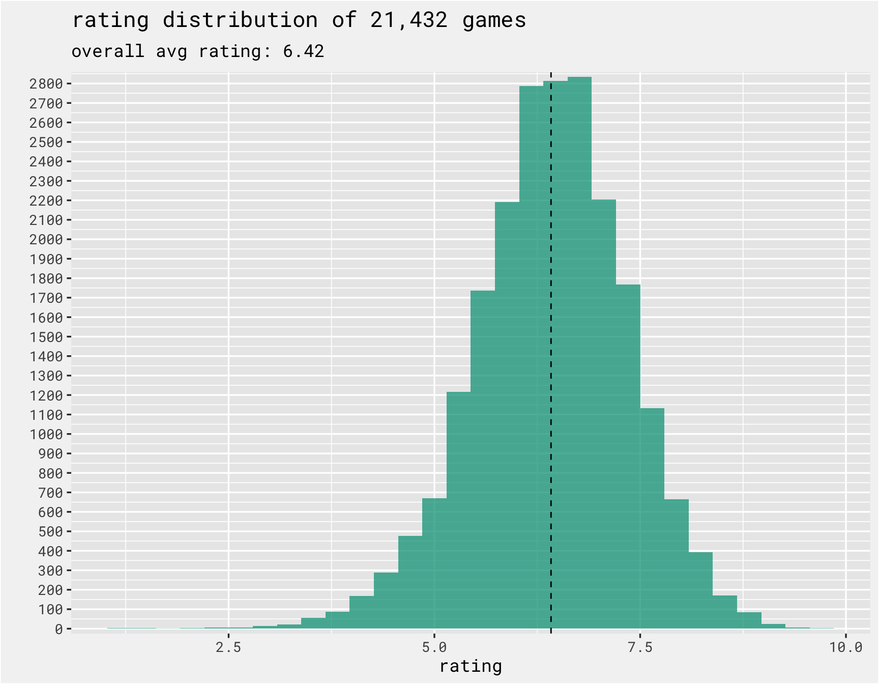
The distribution of the outcome variable, ratings, is somewhat normally distributed with a mean rating of 6.42 out of 10.
n_games <-
  ratings %>%
  distinct(name) %>%
  nrow()

overall_avg <-
  ratings %>%
  summarise(mean_rating = mean(average, na.rm = T)) %>%
  pull(mean_rating)

ratings %>%
  ggplot(aes(x = average)) +
  geom_histogram(alpha = .75, fill = bg_green) +
  bg_theme(base_size = 13) +
  geom_vline(aes(xintercept = mean(average)), linetype = 'dashed') +
  scale_y_continuous(expand = c(0, 25), breaks = seq(0, 3000, 100)) +
  labs(x = "rating", y = '', title =  paste("rating distribution of", format(n_games, big.mark = ','),
                                            "games"),
       subtitle = paste("overall avg rating:", round(overall_avg, 2)))
Here we can dive into the category column. First we combine the ratings data with the details and then tokenize the category column into individual rows per category descriptor. This wirll help form the basis of the text recipe developed later on.
combined <-
  ratings %>%
  inner_join(., details %>% select(-num), by = c("id")) %>%
  select(-c(url, rank, bayes_average, users_rated, yearpublished, thumbnail, primary,
            boardgameexpansion, boardgameimplementation, boardgamedesigner, description,
            boardgamepublisher,boardgameartist, boardgamefamily, boardgamemechanic,
            owned, trading, wanting, wishing, minplaytime, maxplaytime, year)) %>%
  select(num, id, name, average, boardgamecategory, everything()) %>%
  rename(category = boardgamecategory) %>%
  mutate(category = str_remove_all(category, "'"),
         category = str_remove_all(category, '"'),
         category = str_replace_all(category, "\\[|\\]", ""),
         category = trimws(category)) %>%
  filter(!(is.na(category)))

tidy_category <-
  combined %>%
  unnest_tokens(word, category)

tidy_category %>%
  count(word, sort = TRUE)
## # A tibble: 113 × 2
##    word         n
##    <chr>    <int>
##  1 game     10882
##  2 card      6402
##  3 wargame   3820
##  4 fantasy   2681
##  5 war       1996
##  6 party     1968
##  7 dice      1847
##  8 fiction   1666
##  9 science   1666
## 10 fighting  1658
## # … with 103 more rows
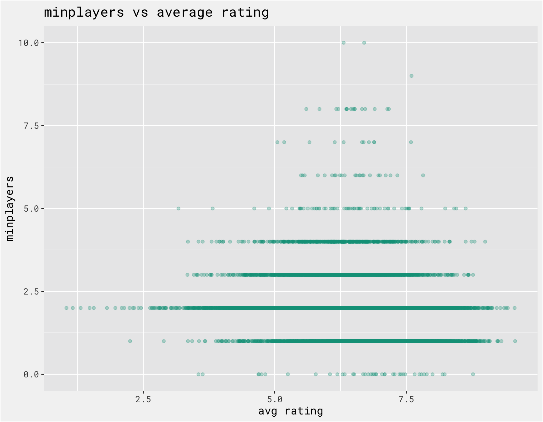
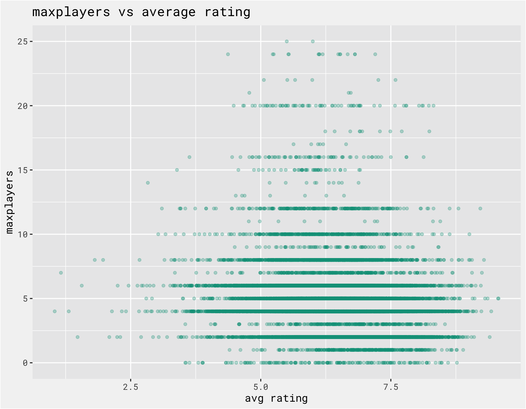
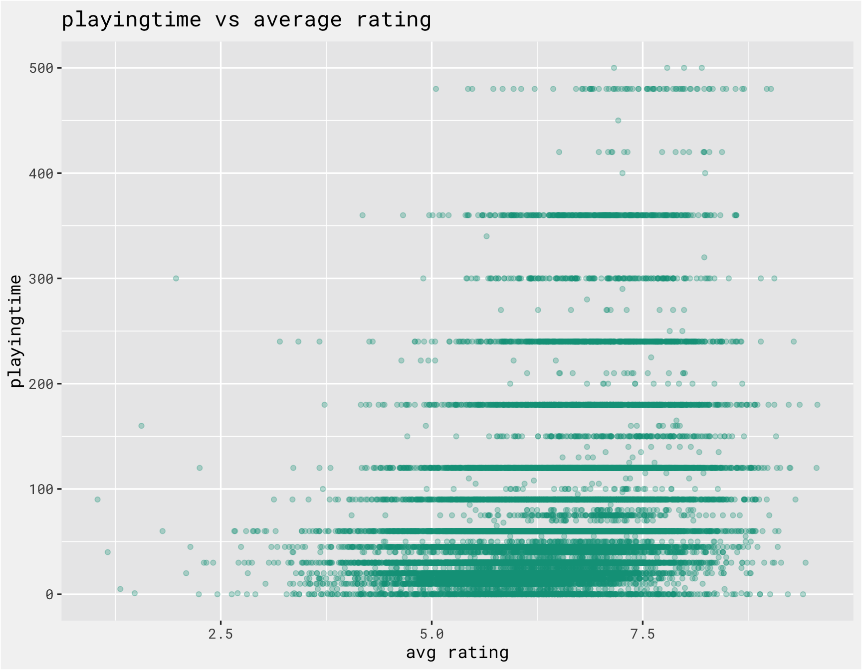
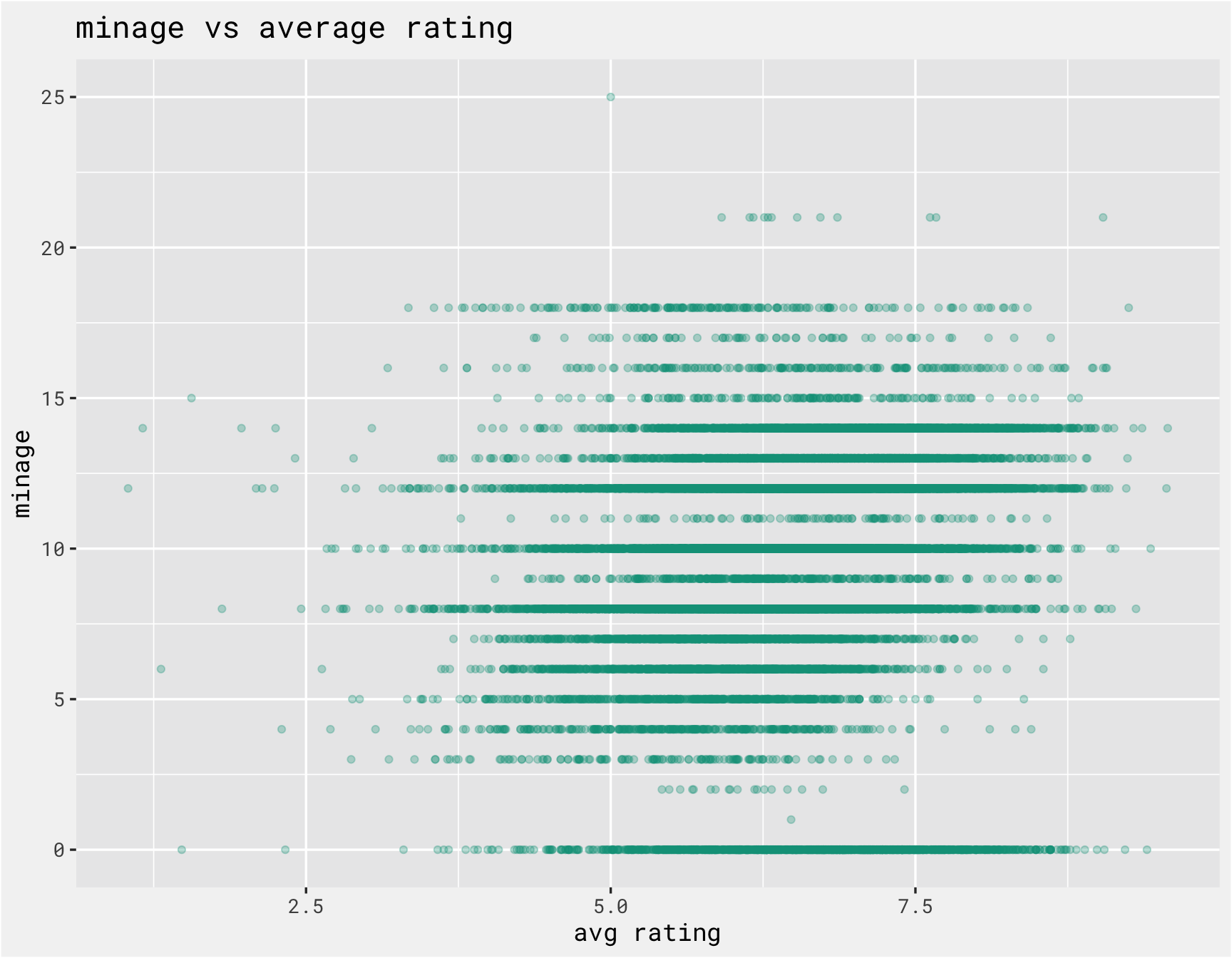
Since we are also including non-text data in the model, we should explore those predictors as well. The function below iterates over the numeric columns and checks the relationship between the numeric columns with the average rating. There are a number of outliers that need to be handled to make the plots more meaningful.
get_scatter <-
  function(data, var){

    variable_filter <-
      if (var == "maxplayers"){
        25
      } else if (var == "playingtime"){
        500
      } else {
        10000000
      }

    data %>%
      select(average, one_of({{var}})) %>%
      rename(variable = 2) %>%
      filter(variable <= variable_filter) %>%
      ggplot(., aes(x = average, y = variable)) +
      geom_point(alpha = .3, color = bg_green) +
      bg_theme(base_size = 13) +
      labs(x = "avg rating", y = var, title = paste(var, "vs average rating"))

  }

numeric_cols <-
  combined %>%
  select(where(is.numeric)) %>%
  select(-c(id, num, average)) %>%
  names

purrr::map(numeric_cols, ~get_scatter(combined, .x))
## [[1]]
##
## [[2]]
##
## [[3]]
##
## [[4]]
Create Some Models
To prep the text data for modeling we can create a matrix with each words TF-IDf value. From the step_tfidf() documentation:
Term frequency-inverse document frequency is the product of two statistics: the term frequency (TF) and the inverse document frequency (IDF).
Term frequency measures how many times each token appears in each observation.
Inverse document frequency is a measure of how informative a word is, e.g., how common or rare the word is across all the observations. If a word >appears in all the observations it might not give that much insight, but if it only appears in some it might help differentiate between observations.
The IDF is defined as follows: idf = log(1 + (# documents in the corpus) / (# documents where the term appears))
Normally we’d used step_tokenfilter() as well, but there are not that many categories so we can use all 113. The important step here is to prep() the recipe and then bake() the results. This sequence of functions applies and executes the recipe, and returns a dataframe ready to be joined with the other predictors.
text_prep <-
  recipe(average ~ num + id + name + category, data = combined) %>%
  update_role(num, id, name, new_role = "ID variables") %>%
  step_tokenize(category) %>%
  step_tfidf(category) %>%
  prep() %>%
  bake(new_data = NULL)

text_prep
## # A tibble: 21,348 × 117
##      num     id name  average tfidf_category_… tfidf_category_… tfidf_category_…
##    <dbl>  <dbl> <fct>   <dbl>            <dbl>            <dbl>            <dbl>
##  1   105  30549 Pand…    7.59                0                0                0
##  2   189    822 Carc…    7.42                0                0                0
##  3   428     13 Catan    7.14                0                0                0
##  4    72  68448 7 Wo…    7.74                0                0                0
##  5   103  36218 Domi…    7.61                0                0                0
##  6   191   9209 Tick…    7.41                0                0                0
##  7   100 178900 Code…    7.6                 0                0                0
##  8     3 167791 Terr…    8.42                0                0                0
##  9    15 173346 7 Wo…    8.11                0                0                0
## 10    35  31260 Agri…    7.93                0                0                0
## # … with 21,338 more rows, and 110 more variables:
## #   tfidf_category_adventure <dbl>, tfidf_category_age <dbl>,
## #   tfidf_category_agents <dbl>, tfidf_category_american <dbl>,
## #   tfidf_category_ancient <dbl>, tfidf_category_and <dbl>,
## #   tfidf_category_animals <dbl>, tfidf_category_arabian <dbl>,
## #   tfidf_category_aviation <dbl>, tfidf_category_base <dbl>,
## #   tfidf_category_based <dbl>, tfidf_category_bluffing <dbl>, …
model_data <-
  combined %>%
  select(-category) %>%
  left_join(., text_prep %>% select(-c(num, name, average)), "id")

model_data
## # A tibble: 21,348 × 121
##      num     id name            average minplayers maxplayers playingtime minage
##    <dbl>  <dbl> <chr>             <dbl>      <dbl>      <dbl>       <dbl>  <dbl>
##  1   105  30549 Pandemic           7.59          2          4          45      8
##  2   189    822 Carcassonne        7.42          2          5          45      7
##  3   428     13 Catan              7.14          3          4         120     10
##  4    72  68448 7 Wonders          7.74          2          7          30     10
##  5   103  36218 Dominion           7.61          2          4          30     13
##  6   191   9209 Ticket to Ride     7.41          2          5          60      8
##  7   100 178900 Codenames          7.6           2          8          15     14
##  8     3 167791 Terraforming M…    8.42          1          5         120     12
##  9    15 173346 7 Wonders Duel     8.11          2          2          30     10
## 10    35  31260 Agricola           7.93          1          5         150     12
## # … with 21,338 more rows, and 113 more variables:
## #   tfidf_category_abstract <dbl>, tfidf_category_action <dbl>,
## #   tfidf_category_adult <dbl>, tfidf_category_adventure <dbl>,
## #   tfidf_category_age <dbl>, tfidf_category_agents <dbl>,
## #   tfidf_category_american <dbl>, tfidf_category_ancient <dbl>,
## #   tfidf_category_and <dbl>, tfidf_category_animals <dbl>,
## #   tfidf_category_arabian <dbl>, tfidf_category_aviation <dbl>, …
Then we prep for modelling by creating splits, resamples, model specifications, recipes (several to compare), and the workflowset:
set.seed(113)
splits <-
  model_data %>%
  initial_split(strata = average)

train <-
  training(splits)
test <-
  testing(splits)

folds <-
  vfold_cv(train, strata = average)
3 recipes are created here with the goal of seeing which combination works the best: one with the just text features, recipe_text and one without any text features, recipe_no_text and then one with all features, recipe_all.
recipe_all <-
  recipe(average ~ ., data = train) %>%
  update_role(num, id, name, new_role = "ID variables") %>%
  step_normalize(minplayers, maxplayers, playingtime, minage)

recipe_text <-
  recipe_all %>%
  step_rm(minplayers, maxplayers, playingtime, minage)

recipe_no_text <-
  recipe_all %>%
  step_rm(starts_with('tfidf'))
svm_spec <-
  svm_linear(cost = tune(),
             margin = tune()
  ) %>%
  set_mode("regression") %>%
  set_engine("LiblineaR")

lasso_spec <-
  parsnip::linear_reg(penalty = tune(),
                      mixture = 1) %>%
  set_engine("glmnet")

mars_spec <-
  parsnip::mars(num_terms = tune(),
                prod_degree = tune()) %>%
  set_mode('regression') %>%
  set_engine("earth")

workflows <-
  workflow_set(
    preproc = list(recipe_all = recipe_all,
                   recipe_text = recipe_text,
                   recipe_numeric = recipe_no_text),
    models = list(svm = svm_spec,
                  lasso = lasso_spec,
                  mars = mars_spec
    ),
    cross = TRUE)

workflows
## # A workflow set/tibble: 9 × 4
##   wflow_id             info             option    result
##   <chr>                <list>           <list>    <list>
## 1 recipe_all_svm       <tibble [1 × 4]> <opts[0]> <list [0]>
## 2 recipe_all_lasso     <tibble [1 × 4]> <opts[0]> <list [0]>
## 3 recipe_all_mars      <tibble [1 × 4]> <opts[0]> <list [0]>
## 4 recipe_text_svm      <tibble [1 × 4]> <opts[0]> <list [0]>
## 5 recipe_text_lasso    <tibble [1 × 4]> <opts[0]> <list [0]>
## 6 recipe_text_mars     <tibble [1 × 4]> <opts[0]> <list [0]>
## 7 recipe_numeric_svm   <tibble [1 × 4]> <opts[0]> <list [0]>
## 8 recipe_numeric_lasso <tibble [1 × 4]> <opts[0]> <list [0]>
## 9 recipe_numeric_mars  <tibble [1 × 4]> <opts[0]> <list [0]>
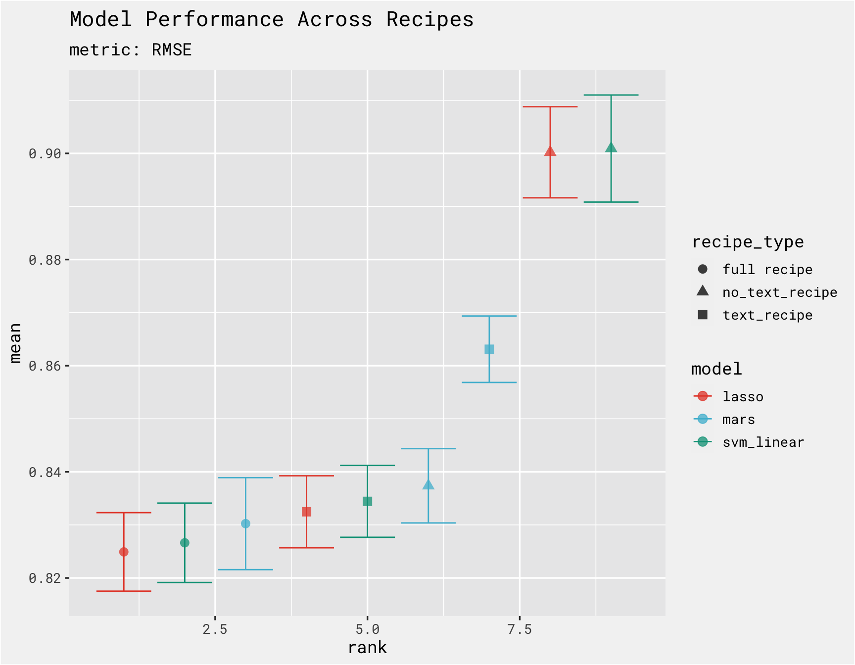
Here we compare the model performance. It looks like the lasso models with the full set of predictors performs the best (circles) and the models without the category text performed the worst (triangles)
grid_ctrl <-
  control_grid(
    save_pred = TRUE,
    allow_par = TRUE,
    parallel_over = "everything",
    verbose = TRUE
  )

cl <-
  makeCluster(10)

doParallel::registerDoParallel(cl)

results <-
  workflow_map(fn = "tune_grid",
               object = workflows,
               seed = 155,
               verbose = TRUE,
               control = grid_ctrl,
               grid = 10,
               resamples = folds,
               metrics = metric_set(rmse, mae)
  )

stopCluster(cl)
rank_results(results, select_best = T) %>%
  mutate(model = ifelse(str_detect(wflow_id, "lasso"), "lasso", model),
         recipe_type = case_when(
           str_detect(wflow_id, "text") ~ "text_recipe",
           str_detect(wflow_id, "all") ~ "full recipe",
           TRUE ~ "no_text_recipe")) %>%
  filter(.metric == 'rmse') %>%
  ggplot(.,aes(x = rank,  y = mean, color = model, shape = recipe_type)) +
  geom_errorbar(aes(ymin = mean - std_err, ymax = mean + std_err)) +
  geom_point(size = 3, alpha = .75) +
  labs(title = "Model Performance Across Recipes", subtitle = "metric: RMSE") +
  bg_theme(base_size = 13) +
  ggsci::scale_color_npg()
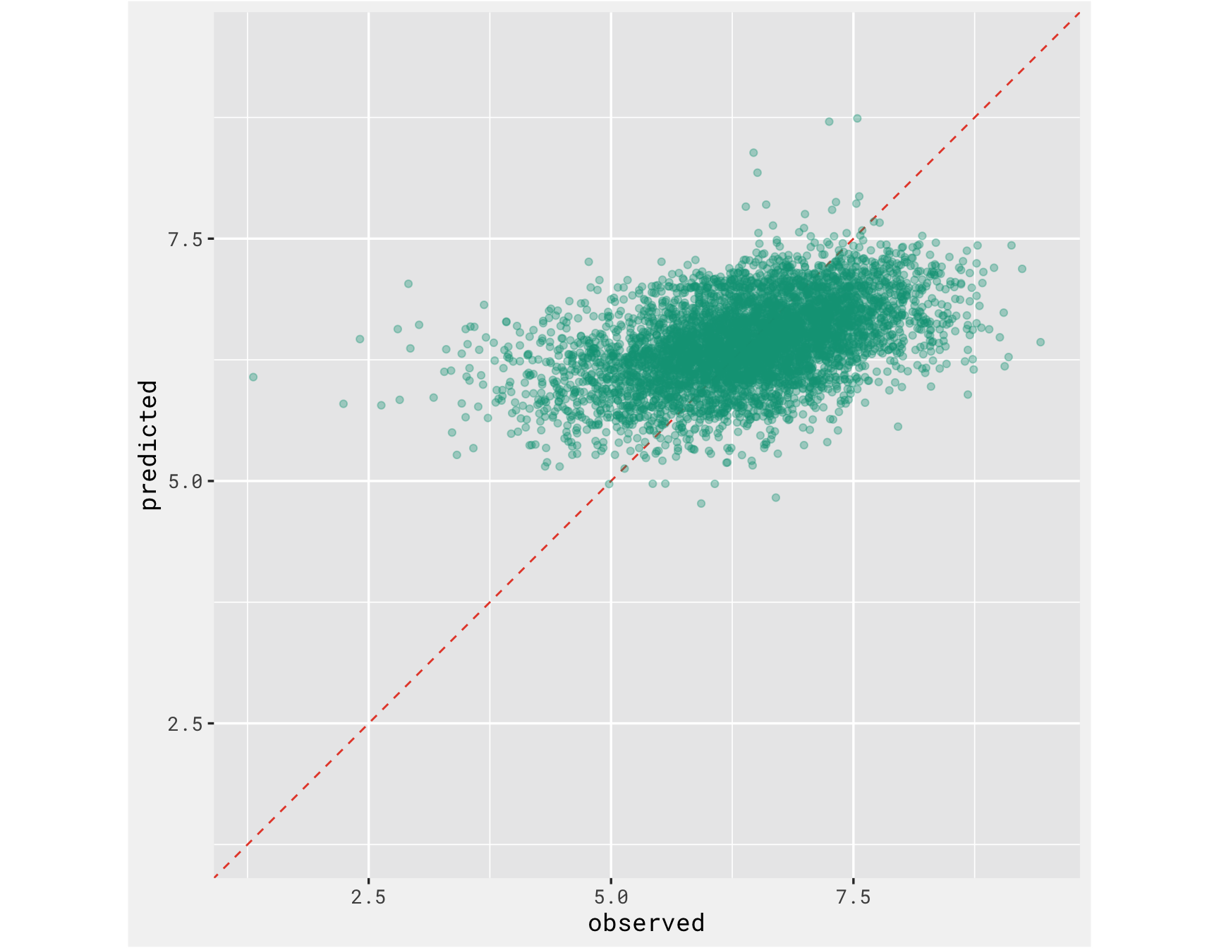
The predicted vs actual performance of the “best” model is not very good. But oh well, and anyway the goal of this post was to combine text data and non-text data into a model.
best_results <-
   results %>%
   extract_workflow_set_result("recipe_all_lasso") %>%
   select_best(metric = "rmse")

best_results
## # A tibble: 1 × 2
##   penalty .config
##     <dbl> <fct>
## 1 0.00350 Preprocessor1_Model08
cl <-
  makeCluster(10)

test_results <-
   results %>%
   extract_workflow("recipe_all_lasso") %>%
   finalize_workflow(best_results) %>%
   last_fit(split = splits)

collect_metrics(test_results)
## # A tibble: 2 × 4
##   .metric .estimator .estimate .config
##   <chr>   <chr>          <dbl> <fct>
## 1 rmse    standard       0.822 Preprocessor1_Model1
## 2 rsq     standard       0.215 Preprocessor1_Model1
stopCluster(cl)

test_results %>%
  collect_predictions() %>%
  ggplot(aes(x = average, y = .pred)) +
  geom_abline(col = "#e64b35", lty = 2) +
  geom_point(alpha = 0.35, color = "#00a087") +
  coord_obs_pred() +
  labs(x = "observed", y = "predicted") +
  bg_theme(base_size = 13) +
  ggsci::scale_color_npg()
- Posted on:
- January 26, 2022
- Length:
- 12 minute read, 2428 words
- Categories:
- tidy tuesday tidymodels data science