Comparing Variability in Ultra Trail Running Results Across Countries

This post looks at a past TidyTuesday data set about ultra trail running. After looking at the data I attempt to quantify and compare the variation in rankings between countries.

Explore the Data

Race data is at the race level; events are made up of races. There can be multiple event observations per year.

race

## # A tibble: 1,207 × 14
##    race_year_id event   race   city  country date       start_time participation
##           <dbl> <chr>   <chr>  <chr> <chr>   <date>     <time>     <chr>        
##  1        68140 Peak D… Mills… Cast… United… 2021-09-03 19:00      solo         
##  2        72496 UTMB®   UTMB®  Cham… France  2021-08-27 17:00      Solo         
##  3        69855 Grand … Ultra… viel… France  2021-08-20 05:00      solo         
##  4        67856 Persen… PERSE… Asen… Bulgar… 2021-08-20 18:00      solo         
##  5        70469 Runfir… 100 M… uluk… Turkey  2021-08-20 18:00      solo         
##  6        66887 Swiss … 160KM  Müns… Switze… 2021-08-15 17:00      solo         
##  7        67851 Salomo… Salom… Foll… Norway  2021-08-14 07:00      solo         
##  8        68241 Ultra … 160KM  Spa   Belgium 2021-08-14 07:00      solo         
##  9        70241 Québec… QMT-1… Beau… Canada  2021-08-13 22:00      solo         
## 10        69945 Bunket… BBUT … LIND… Sweden  2021-08-07 10:00      solo         
## # … with 1,197 more rows, and 6 more variables: distance <dbl>,
## #   elevation_gain <dbl>, elevation_loss <dbl>, aid_stations <dbl>,
## #   participants <dbl>, year <dbl>

Example data for Run Rabbit Run event:

race %>% 
  filter(event == "RUN RABBIT RUN") %>%
  select(event, race, year) %>% 
  arrange(year) %>%
  add_table()

race %>% 
  select(event, race, participants) %>%
  distinct() %>%
  arrange(desc(participants)) %>%
  head(10) %>%
  add_table()

Ranking data is at the racer level; racers can appear more than once:

ultra_rankings 

## # A tibble: 137,803 × 8
##    race_year_id  rank runner     time     age gender nationality time_in_seconds
##           <dbl> <dbl> <chr>      <chr>  <dbl> <chr>  <chr>                 <dbl>
##  1        68140     1 VERHEUL J… 26H 3…    30 M      GBR                   95725
##  2        68140     2 MOULDING … 27H 0…    43 M      GBR                   97229
##  3        68140     3 RICHARDSO… 28H 4…    38 M      GBR                  103747
##  4        68140     4 DYSON Fio… 30H 5…    55 W      GBR                  111217
##  5        68140     5 FRONTERAS… 32H 4…    48 W      GBR                  117981
##  6        68140     6 THOMAS Le… 32H 4…    31 M      GBR                  118000
##  7        68140     7 SHORT Deb… 33H 3…    55 W      GBR                  120601
##  8        68140     8 CROSSLEY … 33H 3…    40 W      GBR                  120803
##  9        68140     9 BUTCHER K… 34H 5…    47 M      GBR                  125656
## 10        68140    10 Hendry Bi… 34H 5…    29 M      GBR                  125979
## # … with 137,793 more rows

ultra_rankings %>%
  group_by(runner, nationality) %>% 
  tally(sort = T) %>%
  head(10) %>%
  add_table()

Variation in Ranking Among Countries

Rankings seem interesting, let’s try and see which countries have runners with the most consistent rankings. First we need to prep the data a little bit. We’ll set a threshold to only include countries where runners from that given country participated in at least 15 races.

country_counts <- 
  ultra_rankings %>%
  select(nationality, race_year_id) %>%
  distinct() %>%
  group_by(nationality) %>%
  tally()

runner_count <-
  ultra_rankings %>%
  select(nationality, runner) %>%
  distinct() %>%
  group_by(nationality) %>%
  tally()

quantile(country_counts$n, probs = seq(0, 1, .10))

##    0%   10%   20%   30%   40%   50%   60%   70%   80%   90%  100% 
##   1.0   1.0   2.0   3.3   8.0  15.5  31.0  41.7  82.4 128.7 700.0

quantile(runner_count$n, probs = seq(0, 1, .10))

##      0%     10%     20%     30%     40%     50%     60%     70%     80%     90% 
##     1.0     1.0     1.0     3.0     6.0    16.0    49.4   143.1   261.6   873.0 
##    100% 
## 20345.0

top_countries <- 
  ultra_rankings %>%
  select(nationality, race_year_id) %>%
  distinct() %>%
  group_by(nationality) %>%
  tally() %>%
  filter(n > 15) %>% 
  pull(nationality)

top_countries <- 
  ultra_rankings %>%
  filter(nationality %in% top_countries) %>%
  na.omit() %>%
  select(nationality, runner) %>%
  distinct() %>%
  group_by(nationality) %>%
  tally() %>% 
  filter(n > 15) %>% 
  pull(nationality)

ultra_rankings %>%
  filter(nationality %in% top_countries) %>%
  filter(!is.na(rank)) %>%
  ggplot(aes(rank)) + 
  geom_histogram() + 
  ggtitle("race rankings") + 
  big_labels

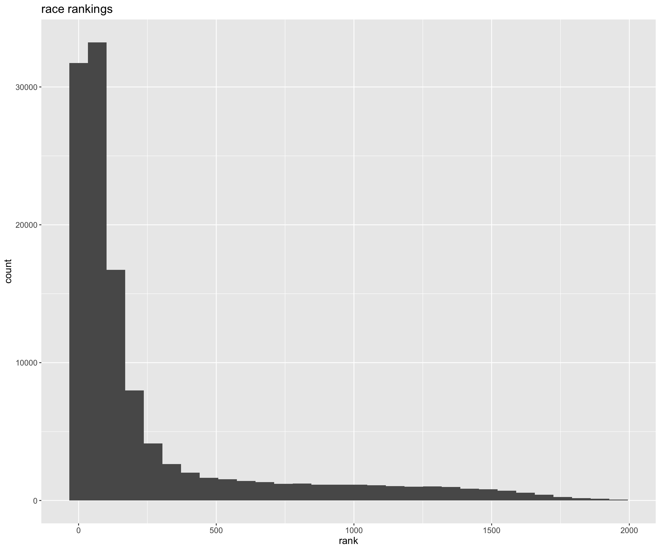
Ranking is highly skewed, so we can use a modified formula for the coefficient of variation meant for log-normal data: $$ {cv_{raw}} = \sqrt{e^{s^2_{ln}} - 1} $$

where \(s_{ln}\) is the sample standard deviation of the data after a natural log transformation. Another alternative we could use the Coefficient of Quartile Variation (see below), but we’ll stick with the modified cv instead.

Coefficient of Quartile Variation

$$ QCV = [(q3 - q1)/(q3 + q1))]*100 $$

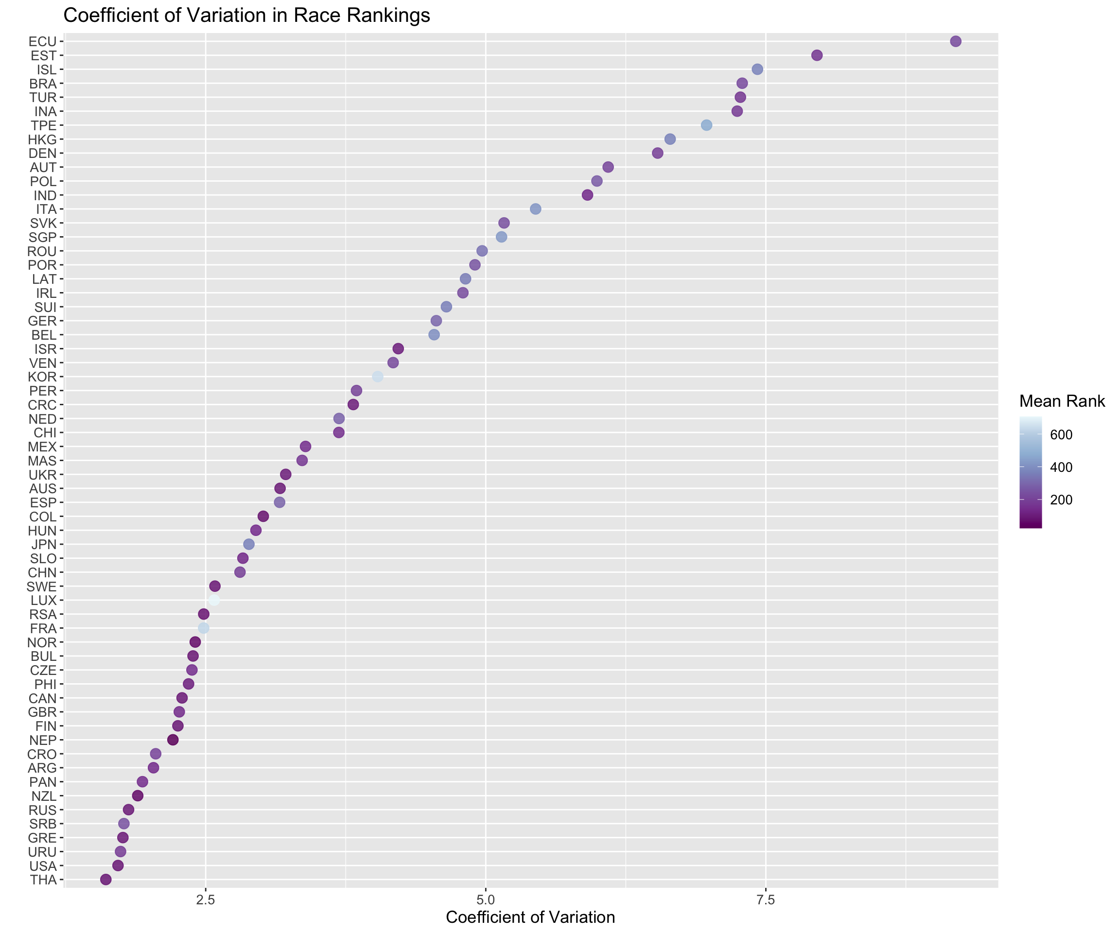
After calculating the CV for log-normal data, we can compare each countries variation. France, Luxembourg and Korea are interesting in that they are relatively consistent, but their median ranks are very high. This suggests racers from these countries get consistently poor results

cv_log <- 
  ultra_rankings %>%
  filter(nationality %in% top_countries) %>%
  filter(!is.na(rank), !(is.na(gender))) %>%
  mutate(log_rank = log(rank)) %>% 
  group_by(nationality) %>% 
  summarise(
    mean_rank = mean(rank, na.rm = T),
    median_rank = median(rank, na.rm = T),
    q3 = quantile(x = rank, probs = .75, na.rm = T),
    q1 = quantile(x = rank, probs = .25, na.rm = T),
    sd_rank = sd(log_rank, na.rm = T),
    cv_log = sqrt((exp(1)^(sd_rank^2)) - 1),
    qcv = ((q3 - q1)/(q3 + q1))*100
  )

cv_log %>%
  ggplot(., aes(x = reorder(nationality, cv_log), y = cv_log, label = round(mean_rank, 2))) + 
  geom_point(size = 3.5, alpha = .85, aes(color = mean_rank)) + 
  scale_color_distiller(direction = -1, palette = "BuPu") +
  coord_flip() +
  labs(y = "Coefficient of Variation", x = "", color = "Mean Rank",
       title = "Coefficient of Variation in Race Rankings") + 
  big_labels

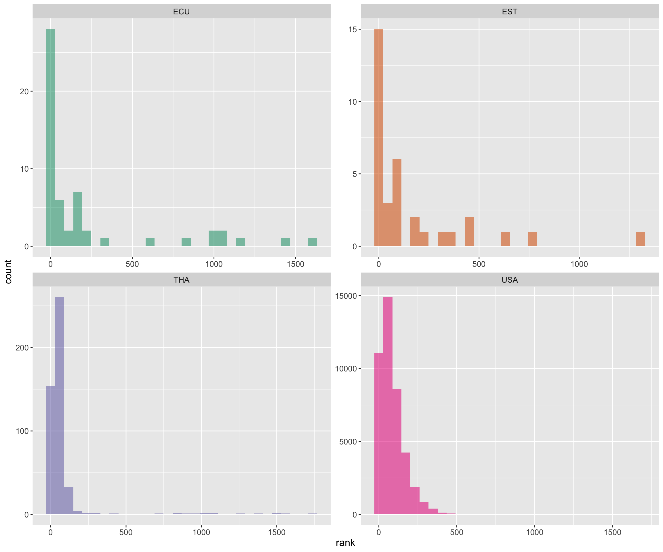
Let’s see if this CV aligns with the distributions of the top 2 and bottom 2 ranked countries. We can compare the ranking distributions of THA and USA with that of EDU and EST. The plot shows that ranking distribution for THA and USA are not as skewed as ECU and EST

ultra_rankings %>%
  filter(nationality %in% top_countries) %>%
  filter(!is.na(rank)) %>%
  filter(nationality %in% c("USA", "THA", "EST", "ECU")) %>% 
  ggplot(aes(x = rank, fill = nationality)) + 
  geom_histogram(position = "stack", show.legend = FALSE, alpha = .55) + 
  facet_wrap(vars(nationality), scales = 'free') +
  big_labels + 
  scale_fill_brewer(palette = "Dark2") 

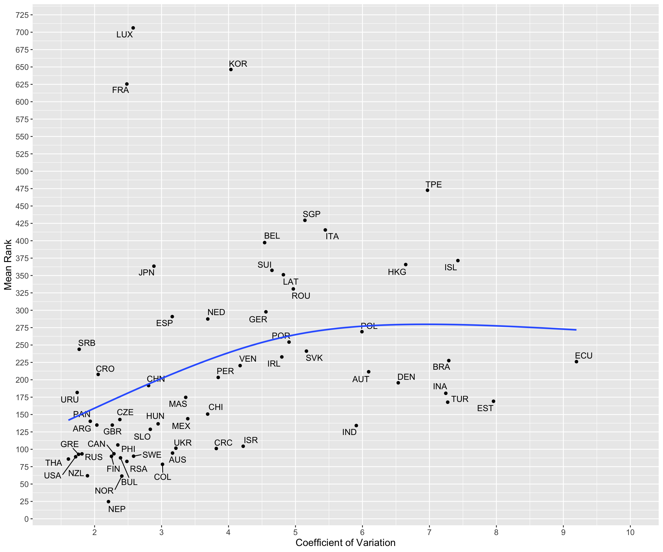
Plotting each country’s mean rank vs CV shows there is slight correlation; countries whose runners are more consistent tend to have better ranking on average.

cv_log %>%
  ggplot(., aes(x = cv_log, y = mean_rank, label = nationality, 2)) + 
  geom_text_repel() + 
  geom_point() + 
  geom_smooth(method = "gam", se = F) +
  labs(x = "Coefficient of Variation", y = "Mean Rank")  + 
  scale_y_continuous(breaks = seq(0, 800, 25)) +
  scale_x_continuous(limits = c(1.5, 10), breaks = seq(0, 10, 1)) + 
  big_labels